商品期货价格数据的降噪处理：以傅立叶变换和卡尔曼滤波变换为例

1. 价格数据降噪处理的重要性

在金融市场中，商品期货的价格往往受到市场波动、噪声以及异常波动的影响。这些噪声可能源于市场的随机性、交易者行为、流动性不足等因素。降噪处理的目的是通过去除价格数据中的短期波动和随机噪声，揭示出价格的长期趋势，从而为投资决策提供更清晰的信号。

降噪处理的意义主要体现在：

• 提高分析的准确性：通过消除价格中的随机波动，投资者能够更加准确地分析市场趋势。
• 减少决策风险：降噪后数据的稳定性提高，有助于投资者减少因噪声引发的错误交易决策。
• 提供稳定的技术指标：许多技术分析指标依赖于平滑处理后的数据，降噪处理能够提高这些指标的有效性。

2. 常见的降噪处理方法

在金融数据处理中，常用的降噪方法可分为常规和复杂处理两类：

• 常规方法：

  • 移动均线（SMA）：最简单且常见的降噪方法，通过取一定窗口内的数据均值来平滑波动，适合短期趋势分析，但滞后性强。

• 复杂方法：

  • 傅立叶变换（Fourier Transform）：通过将时间序列转换为频域信号，并去除高频噪声，从而达到降噪目的。适合处理周期性信号。
  • 卡尔曼滤波（Kalman Filter）：动态优化每个时间点的估计值，通过引入过程方差和测量方差，能适应数据中的非线性变化，适合实时动态数据的降噪。
  • 热方程处理：通过对数据的扩散效应模拟实现平滑效果，较为复杂，适合对多维数据进行处理。

在接下来的部分中，将展示三种典型的降噪方法，包括移动均线、傅立叶变换和卡尔曼滤波，并对其优缺点进行比较。

3. 三种降噪方法的展示

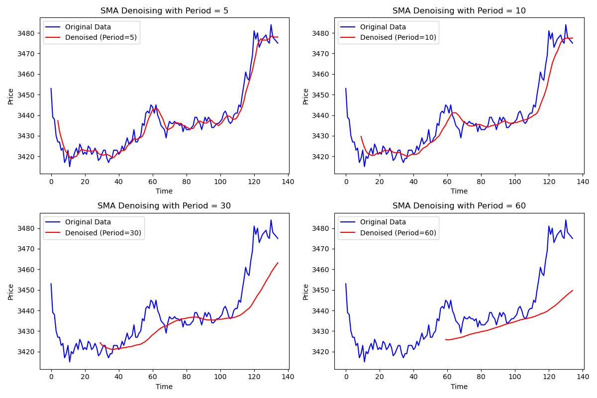
（1）移动均线（SMA）

移动均线通过计算固定周期内的平均值，来平滑原始价格数据，减小短期波动的影响。它的优点是简单易用，但缺点是会引入滞后性，导致对市场变化的响应较慢。

'''backtest
start: 2024-10-10 00:00:00
end: 2024-10-10 09:15:00
period: 1m
basePeriod: 1m
exchanges: [{"eid":"Futures_CTP","currency":"FUTURES"}]
args: [["ffthre",0.1]]
'''

import numpy as np
import pandas as pd
import matplotlib.pyplot as plt


# 移动均线函数
def calSMA(time_series, period):

    moveingAve = TA.MA(time_series, period)

    return moveingAve


def main():
   
    while True:
        r = exchange.GetRecords('rb2501')
        data = pd.DataFrame(r)
        time_series = data['Close'].values
        data['Time'] = range(len(data))

        # 设置不同的周期
        periods = [5, 10, 30, 60]

        plt.figure(figsize=(12, 8))

        # 对不同周期进行降噪并可视化
        for i, period in enumerate(periods):

            sma_time_series = calSMA(time_series, periods[i]) 
            
            plt.subplot(2, 2, i + 1)
            plt.plot(data['Time'], time_series, label='Original Data', color='blue')
            plt.plot(data['Time'], sma_time_series, label=f'Denoised (Period={period})', color='red')
            plt.xlabel('Time')
            plt.ylabel('Price')
            plt.title(f'SMA Denoising with Period = {period}')
            plt.legend()

        plt.tight_layout()
        plt.show()

        LogStatus(plt)

        Sleep(1000 * 10)

原理说明：移动均线对每个时间点的值取前N个点的平均，平滑短期波动，但引入滞后。

滞后性分析：随着周期的增加，滞后性也会增加，导致趋势信号的延迟。

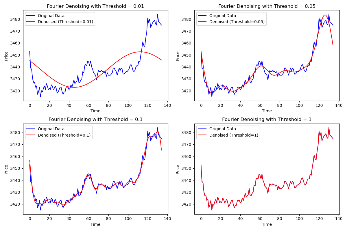
（2）傅立叶变换（FFT）

傅立叶变换将价格数据从时域转换到频域，以便识别其中的周期性成分。通过设置频率阈值，可以过滤掉高频噪声，仅保留低频的趋势信息。

'''backtest
start: 2024-10-10 00:00:00
end: 2024-10-10 09:15:00
period: 1m
basePeriod: 1m
exchanges: [{"eid":"Futures_CTP","currency":"FUTURES"}]
args: [["ffthre",0.1]]
'''
import numpy as np
import pandas as pd
import matplotlib.pyplot as plt
from scipy.fftpack import fft, ifft

def fftransform(time_series, ffthreshold):

    # 进行傅里叶变换
    fft_values = fft(time_series)
    frequencies = np.fft.fftfreq(len(time_series))

    # 复制傅里叶变换值，进行降噪处理
    filtered_fft_values = np.copy(fft_values)
    # 根据阈值设置保留的频率范围，超过阈值的频率被设为 0
    filtered_fft_values[np.abs(frequencies) > ffthreshold] = 0
    
    # 进行逆傅里叶变换并提取实部（去掉复数部分）
    filtered_time_series = ifft(filtered_fft_values)
    filtered_time_series = np.real(filtered_time_series)

    return filtered_time_series


def main():
   
    while True:
        r = exchange.GetRecords('rb2501')
        data = pd.DataFrame(r)
        time_series = data['Close'].values
        data['Time'] = range(len(data))

        # 设置不同的阈值
        thresholds = [0.01, 0.05, 0.1, 1]

        plt.figure(figsize=(12, 8))

        # 对不同阈值进行降噪并可视化
        for i, threshold in enumerate(thresholds):

            filtered_time_series = fftransform(time_series, thresholds[i]) 
            
            plt.subplot(2, 2, i + 1)
            plt.plot(data['Time'], time_series, label='Original Data', color='blue')
            plt.plot(data['Time'], filtered_time_series, label=f'Denoised (Threshold={threshold})', color='red')
            plt.xlabel('Time')
            plt.ylabel('Price')
            plt.title(f'Fourier Denoising with Threshold = {threshold}')
            plt.legend()

        plt.tight_layout()
        plt.show()

        LogStatus(plt)

        Sleep(1000 * 10)

原理说明：傅立叶变换通过频域分析可以有效地分离噪声和趋势。较高的频率对应着噪声，较低的频率对应着长期趋势。傅立叶变换将数据从时间域转换到频域，保留低频信息，去除高频噪声，通过逆变换恢复平滑的时间序列。对周期性信号效果良好。而：对于非周期性信号，处理效果有限。

参数解释：阈值越低，保留的频率成分越多，数据的波动细节更多，降噪效果较弱。阈值越高，保留的频率成分越少，数据变得更加平滑，降噪效果更显著。

图像解释：从图中可以看出，随着阈值的增加，平滑程度增强，降噪效果更为显著。低阈值保留了更多细节，高阈值则更好地滤除了噪声。

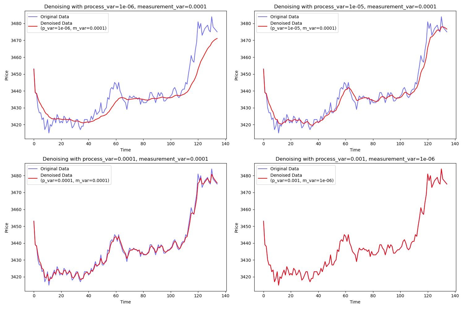
（3）卡尔曼滤波（Kalman Filter）

卡尔曼滤波是一种自适应的降噪方法，能够通过动态调整状态估计来跟踪数据的真实趋势。

'''backtest
start: 2024-10-10 00:00:00
end: 2024-10-10 09:15:00
period: 1m
basePeriod: 1m
exchanges: [{"eid":"Futures_CTP","currency":"FUTURES"}]
args: [["ffthre",0.1]]
'''

import numpy as np
import pandas as pd
import matplotlib.pyplot as plt

# Kalman 滤波器函数，带有可调的过程方差和测量方差参数
def kalman_filter(data, process_variance=1e-5, measurement_variance=0.01**2):
    """
    使用指定的过程方差和测量方差对输入数据进行 Kalman 滤波处理。
    
    :param data: 需要降噪的一维数据（如收盘价数组）。
    :param process_variance: 过程方差（默认值=1e-5）。
    :param measurement_variance: 测量方差（默认值=0.01^2）。
    :return: 使用 Kalman 滤波器处理后的降噪数据。
    """
    n = len(data)
    
    # 初始化状态和协方差
    estimated_state = np.zeros(n)  # 存储每个时刻的状态估计
    estimated_error_covariance = np.zeros(n)  # 存储每个时刻的估计误差协方差
    
    # 对初始状态和初始协方差进行猜测
    estimated_state[0] = data[0]  # 初始状态估计设为第一个数据点
    estimated_error_covariance[0] = 1.0  # 初始估计误差设为 1.0
    
    # 遍历每个数据点
    for i in range(1, n):
        # 预测步骤
        predicted_state = estimated_state[i-1]  # 预测的下一个状态等于前一个估计状态
        predicted_error_covariance = estimated_error_covariance[i-1] + process_variance  # 预测的误差协方差
    
        # 更新步骤
        kalman_gain = predicted_error_covariance / (predicted_error_covariance + measurement_variance)  # 计算卡尔曼增益
        estimated_state[i] = predicted_state + kalman_gain * (data[i] - predicted_state)  # 更新状态估计
        estimated_error_covariance[i] = (1 - kalman_gain) * predicted_error_covariance  # 更新误差协方差
    
    return estimated_state  # 返回降噪后的状态估计值


def main():
    while True:
        r = exchange.GetRecords('rb2501')
        data = pd.DataFrame(r)
    
        time_series = data['Close'].values  # 取出收盘价数据

        data['Time'] = range(len(data))  # 为时间轴创建索引

        # 不同的过程方差和测量方差组合
        variance_settings = [
            (1e-6, 0.01**2),
            (1e-5, 0.01**2),
            (1e-4, 0.01**2),
            (1e-3, 0.001**2),
        ]

        # 可视化原始数据和不同方差下的降噪数据
        plt.figure(figsize=(15, 10))
        for i, (p_var, m_var) in enumerate(variance_settings):
            denoised_data = kalman_filter(time_series, process_variance=p_var, measurement_variance=m_var)
            
            # 在不同的子图中绘制不同方差下的降噪效果
            plt.subplot(2, 2, i+1)
            plt.plot(data['Time'], time_series, label='Original Data', color='blue', alpha=0.6)
            plt.plot(data['Time'], denoised_data, label=f'Denoised Data\n(p_var={p_var}, m_var={m_var})', color='red')
            plt.xlabel('Time')
            plt.ylabel('Price')
            plt.title(f'Denoising with process_var={p_var}, measurement_var={m_var}')
            plt.legend()

        plt.tight_layout()  # 自动调整子图布局
        plt.show()  # 显示图像

        LogStatus(plt)

        Sleep(1000 * 10)

原理说明：卡尔曼滤波通过递归计算来估计当前时刻的真实状态，并且能够动态调整对噪声的敏感度。卡尔曼滤波通过动态更新状态估计值和误差协方差，适应价格数据的动态变化，能实现对数据实时降噪。它适合实时数据，能跟踪数据变化。但是参数设置复杂，对噪声特性敏感。

参数解释：过程方差（process_variance）越小，卡尔曼滤波对变化的敏感度越低，滤波效果更强。测量方差（measurement_variance）控制对测量数据的信任程度。

图像解释：不同的方差组合下，卡尔曼滤波会产生不同程度的平滑效果。较小的过程方差使得数据更加平滑，而较大的过程方差则保留了更多的原始波动信息。

4. 结论

通过对比移动均线、傅立叶变换和卡尔曼滤波，我们可以发现：

• 移动均线实现简单，但滞后性强；
• 傅立叶变换能够有效去除高频噪声，但选择适当的频率阈值很重要；
• 卡尔曼滤波能够自适应调整噪声的影响，效果较为灵活。

5. 数据获取的可靠性

有的同学可能会担心，使用这些降噪方法时是否会涉及未来数据。在优宽量化平台上，您完全可以放心，因为数据的获取是基于固定时间点逐步更新的，而不是一次性地进行更新。这种设计确保了策略在应用降噪处理时，仅依赖历史数据和实时更新的信息，而不会使用到未来数据，从而保持数据的真实性和策略的有效性。因此，您可以安心地在策略中运用这些降噪方法，以提高交易决策的准确性和稳健性。

6. 策略应用

文章最后放一个小彩蛋，使用降噪过后的数据进行双均线策略，对比原始的均线策略效果确实有所提升。大家可以以此为思路，开发更多应用。

'''backtest
start: 2024-09-01 00:00:00
end: 2024-09-30 23:59:59
period: 1h
basePeriod: 1m
exchanges: [{"eid":"Futures_CTP","currency":"FUTURES"}]
args: [["ffthre",0.05]]
'''

import numpy as np
import pandas as pd
from scipy.fftpack import fft, ifft

ffthreshold = 0.05
slowPeriod = 60
fastPeriod = 20

def main():

    def callBack_CTA(st):

        data = pd.DataFrame(st["records"])
        
        time_series = data['Close'].values
        data['Time'] = range(len(data))

        # 进行傅里叶变换
        fft_values = fft(time_series)
        frequencies = np.fft.fftfreq(len(time_series))

        # 复制傅里叶变换值，进行降噪处理
        filtered_fft_values = np.copy(fft_values)
        # 根据阈值设置保留的频率范围，超过阈值的频率被设为 0
        filtered_fft_values[np.abs(frequencies) > ffthreshold] = 0
        
        # 进行逆傅里叶变换并提取实部（去掉复数部分）
        filtered_time_series = ifft(filtered_fft_values)
        filtered_time_series = np.real(filtered_time_series)

        fftvalue = filtered_time_series.tolist()

        emaSlow = TA.EMA(fftvalue, slowPeriod)
        emaFast = TA.EMA(fftvalue, fastPeriod)
        cross = ext.Cross(emaFast, emaSlow)

        ext.PlotRecords(st["records"], "原始均线")
        ext.PlotLine( "傅立叶变换",fftvalue[-1])
        
        if st["position"]["amount"] <= 0 and cross > 2:
            Log("金叉周期", cross, "当前持仓：", st["position"])
            return 2 if st["position"]["amount"] < 0 else 1
        elif st["position"]["amount"] >= 0 and cross < -2:
            Log("死叉周期", cross, "当前持仓：", st["position"])
            return -2 if st["position"]["amount"] > 0 else -1
    
    ret = ext.CTA("sc2411", callBack_CTA)

注：策略需要点击交易和画图模版类库进行使用。

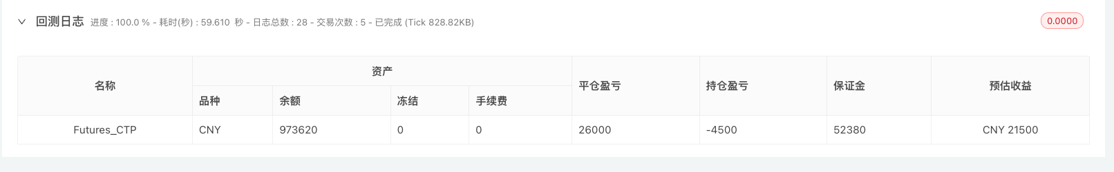
原始均线策略收益

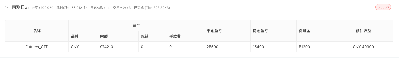
降噪均线策略收益