概述
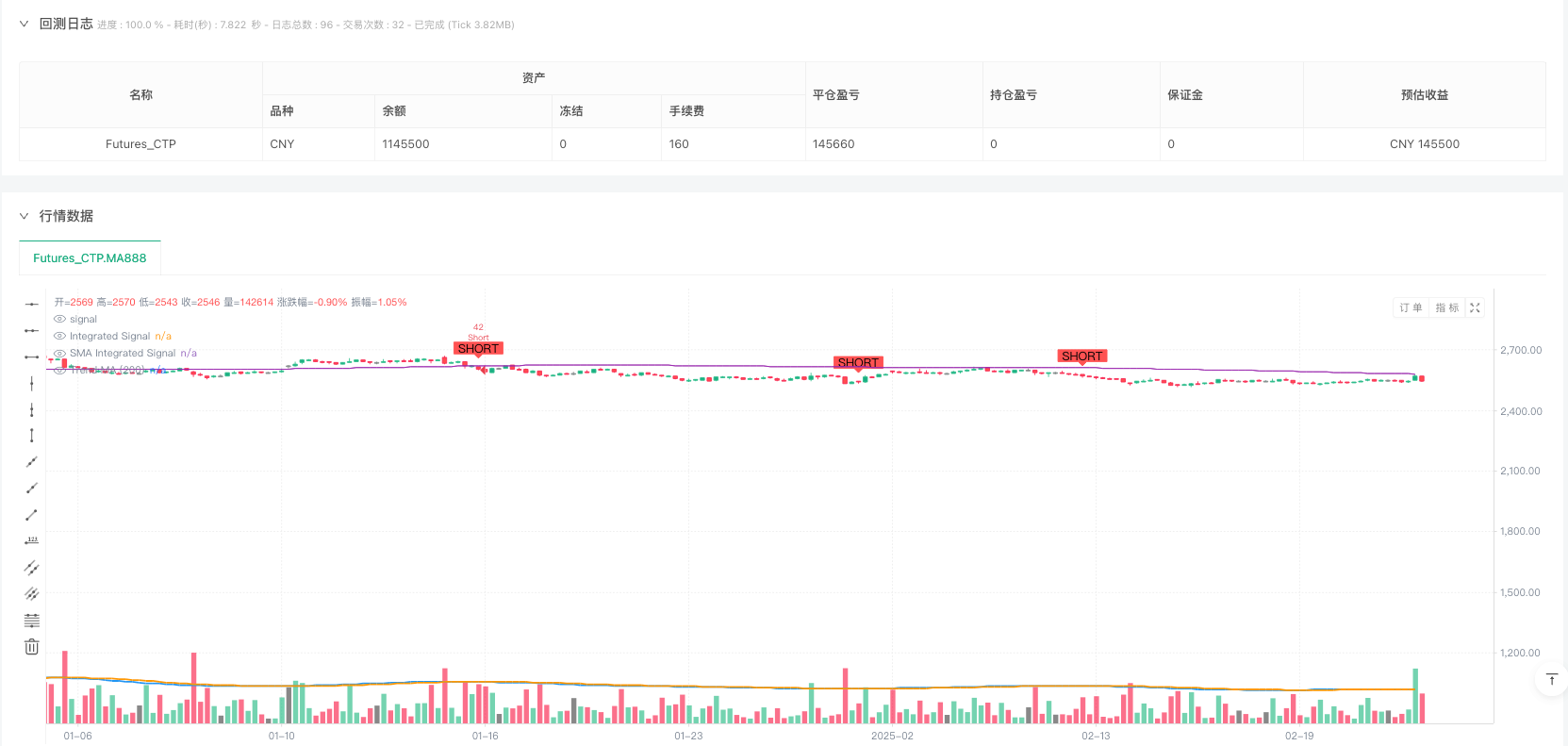
该策略是一个基于Nadaraya-Watson核回归的多维度交易系统,通过整合技术、情绪、超感和意向四个维度的市场信息,形成综合信号来指导交易决策。策略采用权重优化方法,对不同维度的信号进行加权处理,并结合趋势和动量过滤器以提高信号质量。系统还包含完整的风险管理模块,通过止损和止盈来保护资金安全。
策略原理
策略的核心是通过Nadaraya-Watson核回归方法对多个维度的市场数据进行平滑处理。具体来说: 1. 技术维度使用收盘价 2. 情绪维度使用RSI指标 3. 超感维度使用ATR波动率 4. 意向维度使用价格与均线偏离度 这些维度经过核回归平滑后,通过预设权重(技术0.4、情绪0.2、超感0.2、意向0.2)进行加权整合,形成最终的交易信号。当整合信号与其移动平均线发生交叉时,结合趋势和动量过滤器确认后发出交易指令。
策略优势
- 多维度分析提供了更全面的市场视角,避免单一指标的局限性
- Nadaraya-Watson核回归能有效降低市场噪音,提供更平滑的信号
- 权重优化机制允许根据市场特征调整各维度的重要性
- 趋势和动量过滤器的加入显著提高了信号质量
- 完善的风险管理系统确保资金安全
策略风险
- 参数优化过度可能导致过拟合
- 多重过滤条件可能错过部分有效信号
- 核回归计算复杂度较高,可能影响实时性能
- 权重分配不当可能削弱某些重要市场信号 缓解措施包括:使用样本外测试验证参数,动态调整过滤条件,优化计算效率,定期评估和调整权重分配。
策略优化方向
- 引入自适应权重系统,根据市场状态动态调整各维度权重
- 开发更智能的过滤机制,平衡信号质量和数量
- 优化Nadaraya-Watson算法实现,提高计算效率
- 加入市场周期识别模块,在不同市场阶段采用不同的参数设置
- 扩展风险管理系统,增加动态止损和仓位管理功能
总结
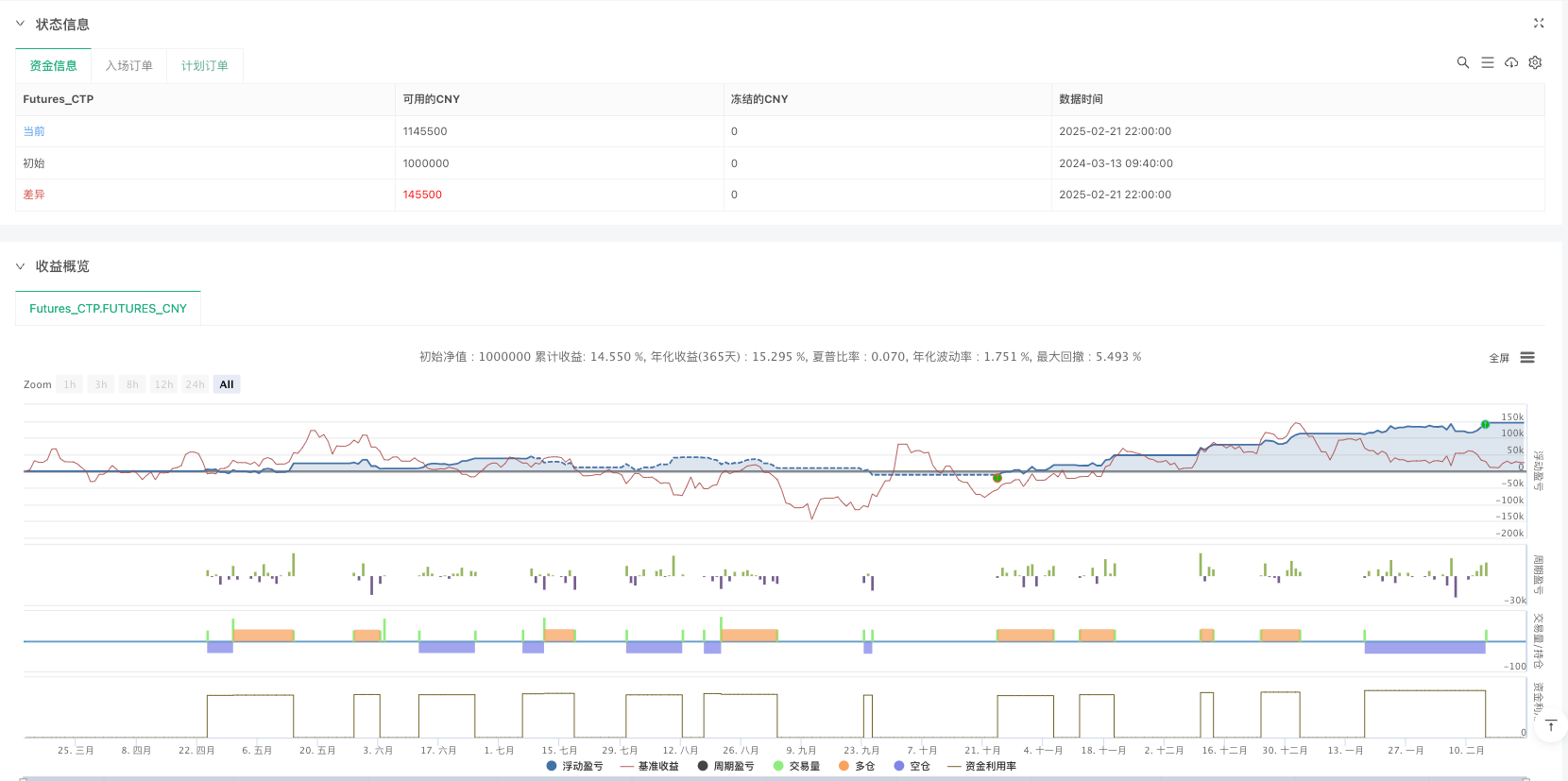
这是一个将数学方法与交易智慧相结合的创新策略。通过多维度分析和先进的数学工具,策略能够捕捉市场的多个层面,提供相对可靠的交易信号。虽然存在一些优化空间,但策略的整体框架是稳健的,具有实际应用价值。
策略源码
/*backtest
start: 2024-03-13 09:40:00
end: 2025-02-23 15:00:00
period: 1h
basePeriod: 1m
exchanges: [{"eid":"Futures_CTP","currency":"FUTURES"}]
*/

//@version=5
strategy("Enhanced Multidimensional Integration Strategy with Nadaraya", overlay=true, initial_capital=10000, currency=currency.USD, default_qty_type=strategy.percent_of_equity, default_qty_value=10)

//────────────────────────────────────────────────────────────────────────────
// 1. Configuration and Weight Optimization Parameters
//────────────────────────────────────────────────────────────────────────────
// Weights can be optimized to favor dimensions with higher historical correlation.
// Base values are maintained but can be fine-tuned.
w_technical   = input.float(0.4,   "Technical Weight",        step=0.05)
w_emotional   = input.float(0.2,   "Emotional Weight",      step=0.05)
w_extrasensor = input.float(0.2,   "Extrasensory Weight", step=0.05)
w_intentional = input.float(0.2,   "Intentional Weight",    step=0.05)

// Parameters for Nadaraya-Watson Smoothing Function:
// Smoothing period and bandwidth affect the "memory" and sensitivity of the signal.
smooth_length = input.int(20, "Smoothing Period", minval=5)
bw_param      = input.float(20, "Bandwidth", minval=1, step=1)

//────────────────────────────────────────────────────────────────────────────
// 2. Risk Management Parameters
//────────────────────────────────────────────────────────────────────────────
// Incorporate stop-loss and take-profit in percentage to protect capital.
// These parameters can be optimized through historical testing.
stopLossPerc   = input.float(1.5, "Stop Loss (%)", step=0.1) / 100   // 1.5% stop-loss
takeProfitPerc = input.float(3.0, "Take Profit (%)", step=0.1) / 100   // 3.0% take-profit

//────────────────────────────────────────────────────────────────────────────
// 3. Additional Filters (Trend and Momentum)
//────────────────────────────────────────────────────────────────────────────
// A long-term moving average is used to confirm the overall trend direction.
trend_length = input.int(200, "Trend MA Period", minval=50)
// RSI is used to confirm momentum. A level of 50 is common to distinguish bullish and bearish phases.
rsi_filter_level = input.int(50, "RSI Confirmation Level", minval=30, maxval=70)

//────────────────────────────────────────────────────────────────────────────
// 4. Definition of Dimensions
//────────────────────────────────────────────────────────────────────────────
tech_series         = close
emotional_series    = ta.rsi(close, 14) / 100
extrasensorial_series = ta.atr(14) / close
intentional_series  = (close - ta.sma(close, 50)) / close

//────────────────────────────────────────────────────────────────────────────
// 5. Nadaraya-Watson Smoothing Function
//────────────────────────────────────────────────────────────────────────────
// This function smooths each dimension using a Gaussian kernel.
// Proper smoothing reduces noise and helps obtain a more robust signal.
nadaraya_smooth(_src, _len, _bw) =>
    if bar_index < _len
        na
    else
        float sumW  = 0.0
        float sumWY = 0.0
        for i = 0 to _len - 1
            weight = math.exp(-0.5 * math.pow(((_len - 1 - i) / _bw), 2))
            sumW  := sumW + weight
            sumWY := sumWY + weight * _src[i]
        sumWY / sumW

//────────────────────────────────────────────────────────────────────────────
// 6. Apply Smoothing to Each Dimension
//────────────────────────────────────────────────────────────────────────────
sm_tech        = nadaraya_smooth(tech_series, smooth_length, bw_param)
sm_emotional   = nadaraya_smooth(emotional_series, smooth_length, bw_param)
sm_extrasens   = nadaraya_smooth(extrasensorial_series, smooth_length, bw_param)
sm_intentional = nadaraya_smooth(intentional_series, smooth_length, bw_param)

//────────────────────────────────────────────────────────────────────────────
// 7. Integration of Dimensions
//────────────────────────────────────────────────────────────────────────────
// The integrated signal is composed of the weighted sum of each smoothed dimension.
// This multidimensional approach seeks to capture different aspects of market behavior.
integrated_signal = (w_technical * sm_tech) + (w_emotional * sm_emotional) + (w_extrasensor * sm_extrasens) + (w_intentional * sm_intentional)
// Additional smoothing of the integrated signal to obtain a reference line.
sma_integrated = ta.sma(integrated_signal, 10)

//────────────────────────────────────────────────────────────────────────────
// 8. Additional Filters to Improve Accuracy and Win Rate
//────────────────────────────────────────────────────────────────────────────
// Trend filter: only trade in the direction of the overall trend, determined by a 200-period SMA.
trendMA = ta.sma(close, trend_length)
// Momentum filter: RSI is used to confirm the strength of the movement (RSI > 50 for long and RSI < 50 for short).
rsi_val = ta.rsi(close, 14)

longFilter  = (close > trendMA) and (rsi_val > rsi_filter_level)
shortFilter = (close < trendMA) and (rsi_val < rsi_filter_level)

// Crossover signals of the integrated signal with its SMA reference.
rawLongSignal  = ta.crossover(integrated_signal, sma_integrated)
rawShortSignal = ta.crossunder(integrated_signal, sma_integrated)
// Incorporate trend and momentum filters to filter false signals.
longSignal  = rawLongSignal and longFilter
shortSignal = rawShortSignal and shortFilter

//────────────────────────────────────────────────────────────────────────────
// 9. Risk Management and Order Generation
//────────────────────────────────────────────────────────────────────────────
// Entries are made based on the filtered integrated signal.
if longSignal
    strategy.entry("Long", strategy.long, comment="Long Entry")
if shortSignal
    strategy.entry("Short", strategy.short, comment="Short Entry")

// Add automatic exits using stop-loss and take-profit to limit losses and secure profits.
// For long positions: stop-loss below entry price and take-profit above.
if strategy.position_size > 0
    strategy.exit("Exit Long", "Long", stop = strategy.position_avg_price * (1 - stopLossPerc), limit = strategy.position_avg_price * (1 + takeProfitPerc))
// For short positions: stop-loss above entry price and take-profit below.
if strategy.position_size < 0
    strategy.exit("Exit Short", "Short", stop = strategy.position_avg_price * (1 + stopLossPerc), limit = strategy.position_avg_price * (1 - takeProfitPerc))

//────────────────────────────────────────────────────────────────────────────
// 10. Visualization on the Chart
//────────────────────────────────────────────────────────────────────────────
plot(integrated_signal, color=color.blue, title="Integrated Signal", linewidth=2)
plot(sma_integrated,      color=color.orange, title="SMA Integrated Signal", linewidth=2)
plot(trendMA,           color=color.purple, title="Trend MA (200)", linewidth=1, style=plot.style_line)
plotshape(longSignal,  title="Long Signal",  location=location.belowbar, color=color.green, style=shape.labelup,   text="LONG")
plotshape(shortSignal, title="Short Signal",  location=location.abovebar, color=color.red,   style=shape.labeldown, text="SHORT")